Inductive PCB rotor position sensor
This is a concept and simulation study for a 21-period, 4 MHz inductive rotor sensor. There is no PCB schematic, layout or hardware. The LTspice circuits and Simulink model are available below; their results do not establish the accuracy of a built sensor.
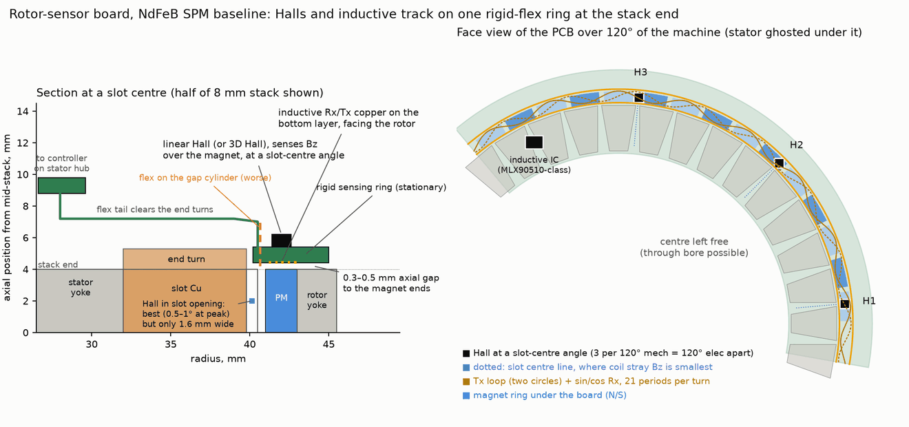
The proposed rigid ring sits at the motor stack end and keeps the shaft bore clear. A copper target modulates the transmit field, and two receive coils read sine and cosine signals. One sensor cycle per pole pair gives electrical angle at standstill, but an output encoder is still needed for joint position. A review found errors in the initial model; the corrections and untested assumptions are listed below.
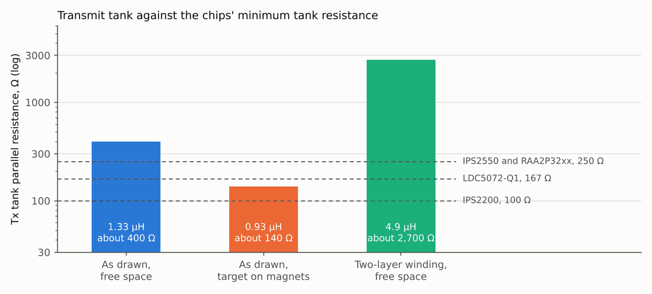
A design review on 12 November 2026 added a thin-sheet eddy-current solve of the coils, the target and the metal near them. It confirmed the coupling the coil model assumed, but it found that the ring position over the magnet ends does not work as drawn. There, the spinning magnets induce about ten times the wanted signal in the receive coils, a target laid on the magnets keeps only 27% of its signal, and the transmit tank falls below the minimum load of most sensor chips. The fix is to move the coils away from the magnets, stand the target at least 1.5 mm off any metal and wind the transmit coil on two layers. The design review section has the numbers.
Simulation files
The LTspice download contains both behavioural .cir netlists, the coil and netlist generators, analysis code and saved parameters. The original results cover the cases without stator interference. The v2 run finished, but its output has not been analysed or accepted.
The Simulink download contains foc_ind_smo.slx, its MATLAB helper scripts and the saved results for three scenarios. The model was saved in R2026a. It tests field-oriented control, observer fusion and fault handling with an assumed sensor budget. It does not establish the accuracy of a manufactured sensor.
Each archive has a README with run notes and a file-hash manifest. The LTspice files are circuit netlists; there is no drawn .asc schematic or PCB layout. The downloads omit raw LTspice waveforms and generated Simulink caches.
The 12 November review found that the coil values in these netlists are out of date. I plan to re-run the v2 netlist once the coil is fixed rather than analyse its current output.
Why 21 sensor periods
The joint motor in my rotor study has 21 pole pairs, which makes an on-axis magnet chip a poor fit. Every mechanical degree of error becomes 21 electrical degrees. The MT6835's factory maximum of ±1° mechanical is ±21° electrical, about 7% less torque per amp, until each unit is calibrated. The magnet also sits on the shaft axis, so it blocks a through bore.
Coil model
The target machine is the rotor study's NdFeB baseline: 36 slots, 42 poles, an 8 mm stack and a 48 V bus. The values come from a Python model of idealised loops. It does not check connected traces, vias or clearances. The status column notes where the 12 November field solve changed the picture; the original values are kept.
| Item | Value | Status |
|---|---|---|
| Ring | r 40.2 to 45 mm | Model input, not checked against the housing |
| Transmit coil | 2 inner + 2 outer turns wound in opposition, 0.3 mm traces, 1 oz copper | Idealised loops |
| Transmit inductance | 1.33 µH, 1.19 nF tank at 4 MHz | Analytic estimate in free space. The solve gives 1.18 µH with the target at 0.5 mm and about 0.93 µH with the target on the magnets |
| Transmit resistance and Q | 1.75 Ω and Q 19, then about 2.8 Ω and Q 12 with a loss allowance | Estimate, proximity loss not extracted. Near the magnets the metal adds 1.1 Ω, so Q is about 6 and the parallel resistance about 140 Ω |
| Receive coils | r = 42.6 ± 1.3 sin(21θ) mm on two layers, sine and cosine | Two-coil design, see corrections |
| Rotor target | 21-period copper pattern shielding 60% of the flux | Assumed at first. Solved for a free-standing target: 1 oz copper acts as a near-perfect shield and adds 0.14 Ω |
| Coupling | About 62.5 nH mutual inductance | Solved: 68 nH at a 0.5 mm gap with a free-standing target, 18.7 nH with the target 0.1 mm over the magnets |
| Coil-shape error | 2.1° electrical peak to peak before calibration | Ideal geometry only. With eddy currents the third harmonic is 0.3%, about 0.17° electrical |
Why not Hall sensors on the rotor magnets
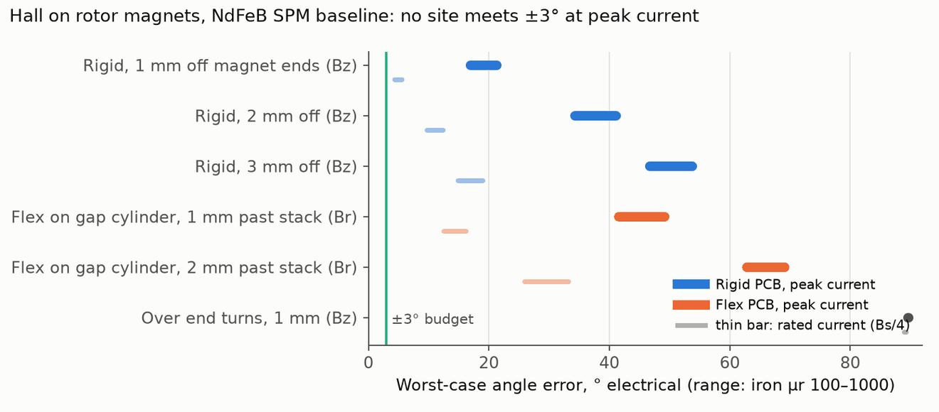
Halls are the cheaper idea, so I checked them with Elmer 3D solves on both rotor types. The stator's own field reaches the sensor and pulls the reading, worst at peak current.
On the NdFeB rotor, a rigid PCB 1 mm off the magnet ends sees ±17 to 21° electrical at peak current. Flex wrapped on the gap cylinder is worse, because it sees as much stray field as magnet field. Over the end turns there is almost no rotor signal at all. The best buildable site is a rigid ring at slot-centre angles within 0.5 mm of the magnets, at ±3 to 4° peak and roughly ±1° at rated current, with a very tight gap. The ferrite spoke rotor gives ±5.6 to 9° at peak.
This does not rule Halls out. These numbers have no current compensation in them, and a measured 12-slot, 10-pole machine in Zhang 2025 dropped from 7.4° to about 0.7° with a feedforward term proportional to q-axis current. I have not simulated that on this 36-slot, 42-pole motor. The solves also use linear iron bracketed at μr 100 and 1000 and an approximate end-turn current sheet.
Carrier circuit in LTspice
The circuit is behavioural. A negative conductance stands in for the oscillator driver, the pickup comes from the coil model's Fourier series, and the ×20 amplifier is ideal. With the stator's stray field switched off, it gives these results at 350 and 1400 Hz electrical:
| Quantity | Result |
|---|---|
| Tank amplitude | 2.95 V peak at 4.0 MHz |
| Demodulated amplitude | 1.78 V |
| Filter group delay | 4.1 µs, 2.1° electrical at 1400 Hz |
| Largest shape error | 1.03° electrical, 4th harmonic, from the ideal coil model |
| Noise at the ADC samples | 0.09 to 0.14° electrical rms |
The stray-field case has no result. Those runs were stopped early, because an ideal amplifier cannot show the problem that matters. By hand, 12 A peak to peak of 40 kHz PWM ripple couples about 0.1 V into a receive coil that carries about 80 mV of signal, which would clip a ×20 stage on a 2.5 V rail. A second netlist adds amplifier rails, a high-pass filter and the higher coil loss. It ran to completion, but its output has not been analysed, so I am not quoting any numbers from it.
The review changed two of these points. The 1.03° shape error comes from the ideal coil model; with real eddy currents the third harmonic is 0.3%, about 0.17° electrical, so I no longer expect an error that large. The model also left out the magnets' own field in the receive coils, which is 5 to 13 times larger than the stator stray field it did include.
Control simulation in Simulink
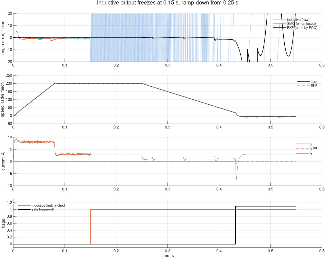
The controller is field-oriented control at 40 kHz with an extended Kalman filter that fuses the inductive angle with a sliding-mode back-EMF observer. The observer fades out at low speed and takes over above about 40 Hz electrical if the inductive channel fails.
| Scenario | Filter angle error | Other |
|---|---|---|
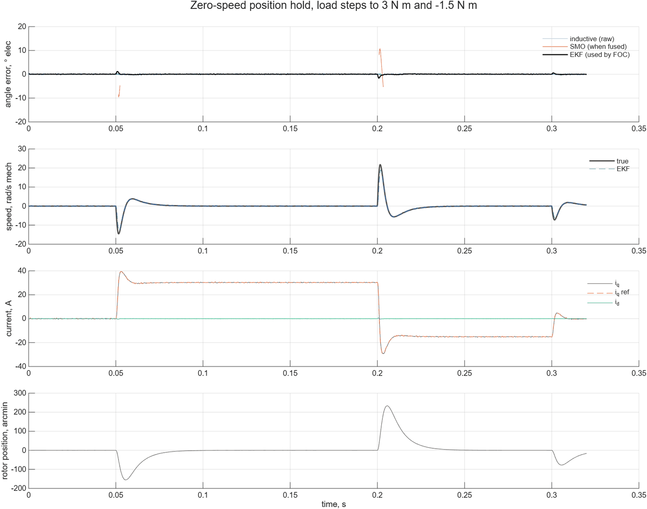
| Zero-speed hold, load steps to 3 N·m and −1.5 N·m | 0.13° electrical rms, 1.6° max | Rotor moves up to 3.9° mechanical and recovers in about 30 ms |
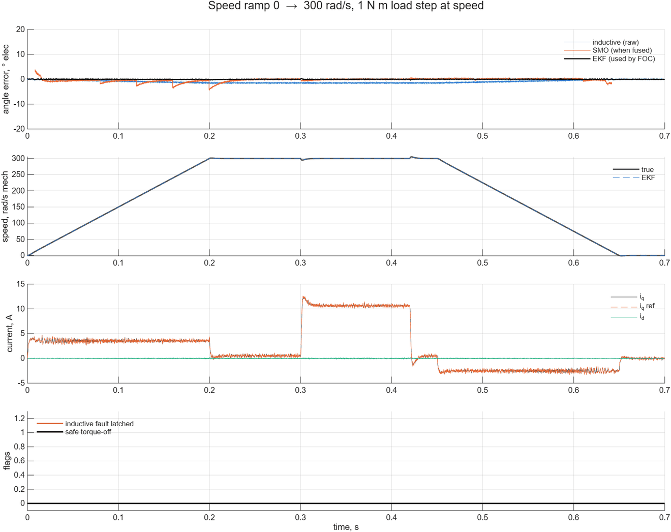
| Ramp to 300 rad/s and back, 1 N·m step at speed | 0.07° rms, 0.36° max | Raw inductive angle 1.1° rms, mostly delay |
| Inductive output frozen at 200 rad/s, then ramp-down | 0.06° rms before the fault | Fault latched in 0.5 ms. Observer alone 0.64° rms, 3.0° max. Torque off at 18 rad/s |
These results show the fusion and fault logic working against the assumed sensor. They say nothing about how accurate a real sensor would be. The sensor model comes from the stray-free LTspice runs, so PWM pickup and clipping are absent. The plant is an averaged inverter with no dead time or ripple, and it assumes 50 µH phase inductance where the rotor study's FEMM model gives about 65 µH. A frozen output at standstill cannot be caught from the angle alone, because no motion contradicts it.
Design review: what the field solve found
On 12 November 2026 I reviewed the concept with a thin-sheet eddy-current solve. The coils are filaments, as in the coil model, and the target and nearby metal are triangle meshes carrying sheet currents, solved at 4 MHz with bfieldtools. It does not compute the transmit trace's own AC resistance, which is still the earlier estimate, it treats steel with one linear permeability, and it has no stator teeth or housing.
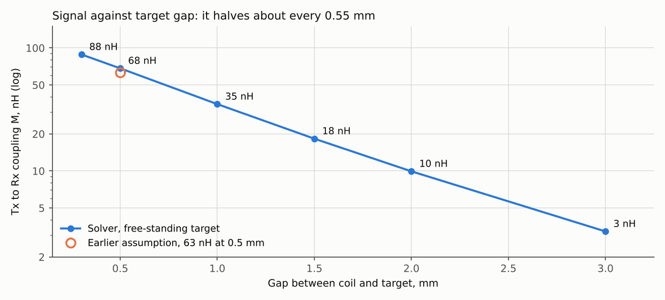
The coil model's main number holds up. The solve gives 68 nH of transmit-to-receive coupling at a 0.5 mm gap, against the 63 nH assumed. The third harmonic is 0.3%, about 0.17° electrical, rather than the 1.7% and roughly 1° the ideal model predicted, so a plain sinusoidal receive outline is good enough for a first board. The 35 µm target thickness is not a problem: the sheet acts as a near-perfect shield and adds only 0.14 Ω to the transmit coil.
The placement is the problem. As drawn, the ring sits 0.4 mm over the magnet ends with the target on the rotor face. That position has three faults the earlier work missed.
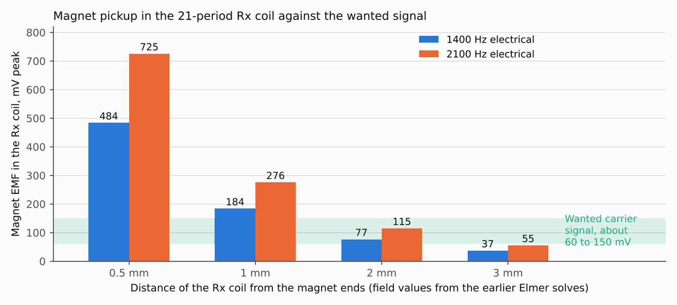
Magnet back-EMF. The receive coil has 21 periods and the rotor has 21 pole pairs, so the coil is a search coil for the magnets' axial leakage field. At the drawn position the magnets induce about 0.5 to 0.7 V at 1.4 to 2.1 kHz, roughly ten times the wanted signal. No earlier model included it: the LTspice model only had the stator's stray field, which is 5 to 13 times smaller. At 3 mm from the magnets the same sum gives 37 to 55 mV. That is far below the carrier frequency, so a chip with a band-pass front end can reject it, but only if it does not overload first.
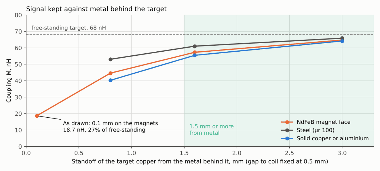
Metal behind the target. A target laid on the magnets keeps 27% of its signal, because the bare metal between the lobes shields the field nearly as well as the copper lobes do. The target copper needs at least 1.5 mm of standoff from any metal, for example a 1.6 mm FR-4 target with copper on the sensor side only.
Transmit tank. With the target on the magnets, the transmit inductance falls from 1.33 to about 0.93 µH and the parallel resistance to about 140 Ω, below the minimum of most candidate chips. The same 2+2 turns on two layers in series give about 4.9 µH and about 2.7 kΩ in free space.
The gap also matters more than my notes assumed. The coupling is 88, 68, 35, 18, 10 and 3 nH at 0.3, 0.5, 1.0, 1.5, 2.0 and 3.0 mm, so the signal halves about every 0.55 mm. The review suggests a nominal gap of 0.5 to 1.0 mm with axial runout under about ±0.15 mm.
| Case (target gap 0.5 mm unless noted) | Tx L, µH | Loss added to Tx, Ω | Coupling M, nH | Share of free-standing |
|---|---|---|---|---|
| No target (free space) | 1.33 | 0 | 0 | |
| Free-standing target | 1.18 | 0.14 | 68 | 100% |
| Free-standing target, 1.0 mm gap | 1.25 | 0.08 | 35 | |
| Free-standing target, 3.0 mm gap | 1.32 | 0.01 | 3 | |
| Target 0.1 mm above magnet face (as drawn) | 0.93 | 1.09 | 18.7 | 27% |
| Target 0.8 mm above magnet face | 1.06 | 0.54 | 44.6 | 65% |
| Target 1.6 mm above magnet face | 1.12 | 0.32 | 57 | 84% |
| Target 1.6 mm above steel | 1.14 | 0.49 | 61 | 89% |
| Target 0.8 mm above solid copper or aluminium | 1.04 | 0.16 | 40 | 59% |
These are solver results on idealised geometry. None of them has been measured.
What the review corrected
A second pass through the sources changed these conclusions. The 12 November design review added the last four rows and the notes marked with its date:
| First pass | Correction |
|---|---|
| The two-coil pattern suits any sensor IC | IPS2200 uses two receive coils, MLX90510 three and MLX90520 six. This pattern only suits the first, or a discrete readout. 12 Nov: TI LDC5072-Q1 and Renesas IPS2550 also use two coils |
| MLX90510's ±0.36° electrical is the expected accuracy | That is the IC's specification. It leaves out errors from a custom target, PCB and mounting. 12 Nov: MLX90510 is no longer the baseline, so this is not the number to beat |
| Coupling k = 4.7% | 4.7% is M/Ltx. Conventional k would be about 7.7% with an assumed 0.5 µH receive coil, and neither is validated |
| About 0.3° electrical calibrated assembly error, scaled from An 2026 | Withdrawn. An 2026 also uses a full-circle ring, not the arc the first pass described, and its tests do not scale linearly to these tolerances |
| Constant 60% target shielding | 35 µm copper at 4 MHz is about one skin depth thick, so this needs a thin-conductor model or a resolved solve. 12 Nov: retired. The test for a thin sheet is its sheet resistance against the field scale, and it passes by over 100 times. The solve shows 1 oz copper acts as a near-perfect shield |
| Filter chain with oversampling and averaging | 18 kHz Butterworth plus an eight-sample average adds about 23.4 µs, and the average alone gives only about 29 dB around the PWM frequency. 12 Nov: with a sensor chip, a single RC near 100 kHz at the ADC pin is enough |
| The Kalman filter can check calibration | It consumes the same sensor. Accuracy needs an independent encoder |
| IPS2200 or MLX90510 as the sensor chip | IPS2200 is listed end of life, and MLX90510 is 5 V only and needs a three-phase coil, so neither is the baseline. The current pick for a first coupon is TI LDC5072-Q1, with Renesas IPS2550 as the alternate. Their datasheet limits still need confirming before ordering |
| Ring 0.4 mm over the magnet ends, target on the rotor face | Does not work as drawn: magnet EMF about ten times the signal, 27% of the target signal left and a transmit tank below most chips' minimum. See the design review section |
| Flex tail carrying the coil signals over the end windings | Dropped. The end turns carry 48 V edges and the full phase current. The chip goes next to the coils, within about 10 mm of the coil exits, and only supply and the demodulated outputs leave the board |
| Single-layer transmit coil, 1.33 µH | Too low and too lossy near metal. The same turns on two layers in series give about 4.9 µH |
Output encoder and next steps
The same approach could read the gearbox output with a two-track 32/31 vernier ring. If each track really held ±0.36° electrical, the fine track would contribute ±0.011° mechanical, with a margin of about 7.8 times on picking the right period. That is a paper bound and leaves out runout, timing skew and coupling between tracks. The ±0.36° is the MLX90510 specification, and that chip is no longer the baseline, so the bound needs redoing for the chosen chip. Using it for gearbox deflection damping depends on noise rather than accuracy, and the gearbox stiffness has not been measured.
The earlier plan was to choose a sensor IC, then run an eddy-current model. The 12 November review did a first pass of both. The next steps now are:
| Step | Why |
|---|---|
| Evaluate putting the coils on the hub controller board, a ring at about 20 to 28 mm radius facing a target on the rotor bell | Removes the flex tail, puts the chip next to the coils and moves them 10 mm or more from the magnets. The period shrinks to about 7 mm, so the signal falls off with gap almost twice as fast |
| FastHenry on the transmit trace | The trace's AC resistance with proximity loss is still an estimate |
| End-winding stray field at that radius, from the existing Elmer model | Not computed yet for the hub position |
| A coupon with the chip, spun with the magnets present | Measures the magnet pickup directly. Only a spin test shows whether the chip's front end tolerates it |
| Accuracy against an independent encoder | The Kalman filter cannot check its own sensor |
Papers
Sources for the sensor study. The collection has 30 entries, including 23 with a checked PDF. The table lists the main references and which parts were reviewed.
| Paper | Used for | Checked |
|---|---|---|
| Kuntz et al. 2025, coupled PCB coil sensors ↗ | Sensor mechanism and simulation method | Design and FEM sections |
| An et al. 2026, misalignment-tolerant eddy-current encoder ↗ | Full-circle coarse and fine tracks, calibration | Architecture, calibration, results |
| Nishiyama et al. 2025, inductive sensor for PMSM rotor angle ↗ | Target overlap as a sweep direction | Full paper |
| Gao et al. 2021, planar inductive absolute angle sensor ↗ | Adjacent-period absolute decoding (63/64) | Architecture, experiment |
| Nauduri et al. 2018, planar inductive sensor for PMSM control ↗ | One-time offset calibration, loaded startup | Implementation, experiments |
| Jow and Ghovanloo 2007, printed spiral coils ↗ | Approximate coil loss model | Equations checked |
| Zhang et al. 2025, armature reaction compensation ↗ | Current feedforward for Hall sensors | Measured result checked |
| Kuntz et al. 2024, multi-winding receiver coils ↗ | Lead for a manufacturable receive coil | Opening sections only |
| Hoxha et al. 2022, PCB rotary sensor optimisation ↗ | Lead for geometry optimisation | Abstract and conclusion only |